Module 3

Module 3: Mathlets in Homework

Each segment of this module consists of sample homework assignments created around one or another of the MIT Mathlets. Each segment is followed by an opportunity for you to discuss this material on the Discussion Forum, and some remarks of my own about the features of the Mathlets and their use that are illuminated by these examples. At the end there are a couple of exercises for you.

1. Outline

This module outline is provided to serve as your guide as you progress through the online content for module 3. It includes of the following:

Outline
Learning Objectives
Mathlets in Homework, Segment 1
- Text of Homework use of Wheel and Taylor Polynomials Mathlets
- Discussion Questions
- Discussion of Segment 1
- Conclusion
Mathlets in Homework, Segment 2
- Text of Homework use of Secant Approximation and Phase Second Order IV Mathlets
- Discussion Questions
- Discussion of Segment 2
Module Conclusion
Exercises
Resources

2. Learning Objectives

After completing this module, the participant will be able to use Mathlets to:

Mix experiment with computation in homework.
Improve student understanding regarding the significance computations in homework.
Increase student enjoyment of homework exercises.

3. Mathlets in Homework, Segment 1

The final use we will look at during this short course is the use of Mathlets as part of homework. Let me introduce you to the idea and benefits of using Mathlets in homework during this next video segment.

Download the transcript for the Mathlets in Homework, Segment 1 video.

First Assignment: Vector Addition

This exercise would be appropriate in a class discussing parametrized curves.

Launch the Wheel Mathlet.

You see a wheel with a light at the end of a spoke. Animate the rolling wheel using the [>>] key. You can return the wheel to the start position using the [<<] key. You can also control $\theta$ directly using the slider.

(a) Adjust the $a$ and $b$ sliders. What does $a$ represent? What does $b$ represent?
(b) You can cause the trajectories of the center of the wheel and the light to be marked by selecting the [trace] key. Give a parametric formula for the location of the center of the wheel (in terms of these parameters) as a function of $\theta$ .
(c) Give a parametric formula for the location of the yellow light as a function of $\theta$ .
(d) You can cause the velocity vector to be shown by selecting the [velocity] key. Are there settings for $a$ , $b$ , and $\theta$ for which the velocity is zero? You may want to discover them using the Mathlet; but then verify your observation mathematically.
(e) By experimenting with the Mathlet, identify situations in which the horizontal component of the velocity vector vanishes. Then verify this observation mathematically.
(f) In fact, what can you say about how the sign of the horizontal component of the velocity vector is related to the position of the light? Again, verify this observation mathematically.

Comments

(a) Just as in a lecture, you have to lead students through the elements of a Mathlet. It is a good idea to encourage students to express the meaning of elements of the Mathlet themselves:

(b)-(c) Do you think that having the parametric expression for the light present on the screen lessens the value of these questions?

(d)-(f) Now we start experimenting. Homework in Mathematics classes often involves somewhat random computations, designed to give the student practice at carrying out some manipulation or algorthm. The Mathlet provides a graphical reason for wanting to do such calculations.

Before moving onto the next project I encourage you to scroll down to the Segment 1 Discussion Questions and post your ideas for incorporating the Taylor Polynomials Mathlet into your courses.

Second Assignment: Taylor Polynomials

Launch the Taylor Polynomials Mathlet.

There is a lot to play with here! When you have explored the Mathlet a little, settle down on the menu item $f(x)=1/(1+x^2)$ .

(a) Compute the full MacLaurin series (the Taylor series at $a=0$ ). Then select $a=0$ on the Mathlet and use the [Terms] key and a large value of $n$ to check your answer.

(b) Set $n=2$ and animate the second order Taylor series by setting $a=-3$ and pressing the [>>] key. You see a family of parabolas. Sometimes they are opening up and sometimes they are opening down. Find (by calculus) the values of $x$ at which these transitions occur. Do these points have a name?

(c) Now set $n=3$ and animate the third order Taylor series. From the Mathlet, observe where the coefficient of the third order term vanishes. What is the name of the graph of the Taylor polynomial at those points? Then compute where those points are.

(d) Now, using the same function, select $a=1$ . The [Terms] readout will display the coefficients in the Taylor series. From these data, predict what the entire Taylor polynomial will be. Then prove your prediction.

Comments

(a) I thought it was important to focus on the Taylor series at a single point, maybe beginning at the point $a=0$ , before moving to the animation offered by this Mathlet.

(b) Perhaps I should have interposed an animation with $n=1$ , to let students see the more familiar tangent line before they see the best approximating parabola. The parabola flattens out to a straight line at the points of inflection. This is what we envision in teaching about points of inflection, but without a tool like this it is hard to convey to the student, and my guess is that identifying the transition from concave to convex with the points of inflection will come as something of a revelation.

(c) Luckily the zeros of $f^{(3)}(x)$ come out nicely, but this is still a substantial computation for beginners, one which might be resented without the payoff of verifying an observation.

(d) This was a surprise to me! You can substitute $x=1+u$ into $f(x)$ , but the result, $1/(2+2u+u^2)$ , does not expand in any very obvious way. With enough insight you can realize that $(2+2u+u^2)(2-2u+u^2)=4+u^4$ , so

$f(x)=\frac{2-2u+u^2}{4+u^4}=\left(\frac{1}{2}-\frac{u}{2}+\frac{u^2}{4}\right)\sum_{k=0}^\infty\left(-\frac{u^4}{4}\right)^k$

agreeing with the coefficients on the Mathlet. It is actually easier to start from the Taylor expansion guessable from the displayed coefficients and work back; so the Mathlet provides a useful hint.

This choice of menu item was rather random; similar exercises could be constructed around any of the others. The last one is the standard example of a $C^\infty$ function which is not real-analytic. It is very interesting to see how the Taylor coefficients all become zero as $x$ decreases to 0. Quite often I find myself surprised and puzzled by behaviors displayed by a Mathlet; this is a good example.

Discussion Questions

Take a few moments to post a response in the following discussion forum. Once you have posted your response, please read and respond to two of your classmates posts.

Here are some examples of homework problems involving various Mathlets.

Module 3 Discussion Question 1: Wheel Project Ideas

Module 3 Discussion Question 2: Taylor Polynomial Project Ideas

4. Mathlets in Lecture, Segment 2

Here are some examples of homework problems involving various Mathlets.

First Assignment: Secant Approximation

This assignment might be given in a calculus course. The early sections would be appropriate when the derivative is being introduced.

Launch the Secant Approximation Mathlet.

Accept the default menu choice $f(x)=\sin(x)$ . Play with the two sliders and the two check boxes.

(a) When $\Delta x=0$ , the yellow secant line disappears. Please explain why.

Set $a=\pi/2$ . (Notice that you can set a slider at a value marked by a hashmark buy clicking on the hashmark.)

(b) What is the slope of the tangent line at this point?

(c) Move the $\Delta x$ slider left and right, and then leave it at $\Delta x=-0.50\pi$ . What is the yellow read-out of the value of the slope of this secant line? What is its actual value?

(d) The claim is that

$\lim_{\Delta x\rightarrow0}\frac{\Delta y}{\Delta x}=0$

Using the Mathlet to gather empirical data, make a table showing how small you have to make $|\Delta x|$ to guarantee that $|\Delta y/\Delta x|<\epsilon$ for the following values of $\epsilon$ : $0.6,0.4,0.2,0.1,0.05,0.02$ .

(e) For this value of $a$ and small $|\Delta x|$ , the slope of the secant is less than the slope of the tangent for $\Delta x>0$ and greater that the slope of the tangent for $\Delta x<0$ . Move the $a$ slider to other positions and observe the relationship between $\Delta y/\Delta x$ and $dy/dx$ at other points. What regularity do you observe? With what other features of the graph does this relationship seem to correlate?

(f) [For classes covering quadratic approximation or Taylor series] Please explain what you observed in (e).

Before moving onto the next project I encourage you to scroll down to the Segment 2 Discussion Questions and post your ideas for incorporating the Secant Approximation Mathlet into your courses.

Second Assignment: Frequency Response

This assignment would be appropriate in an engineering-oriented ordinary differential equations class.

Launch the Amplitude and Phase: Second Order IV Mathlet.

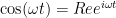
This Mathlet deals with a spring-mass-dashpot system. The input signal is a force acting directly on the mass, given by $F(t)=\cos(\omega t)$ ; the system response is the displacement of the mass from its neutral position. We are interested only in the periodic system response.

Observe the various sliders and their functions.

(a) Set $m=0.50$ , $b=0.33$ , and $k=0.50$ . Sweep the angular frequency from $\omega=0$ to $\omega=4$ . Use the Mathlet to give a qualitative description of the system response, as it relates to the input signal: is its amplitude greater than or less than that of the input signal? is it in phase or does it lag behind? These observations will depend upon the value of $\omega$ . What happens when $\omega$ is small? large?
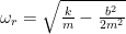
(b) Still with these settings, it appears that there is a particular value of the input angular frequency $\omega$ for which the amplitude of the system response is maximal. This is the near-resonant frequency, written $\omega_r$ . Estimate $\omega_r$ from the Mathlet, and the amplitude of the corresponding system response. It may help to invoke the Bode plots: the upper one shows the amplitude of the system response as a function of $\omega$ . Then compute $\omega_r$ and the amplitude of the near resonant system response exactly (using $b=\frac{1}{3}$ , which was approximated by $b=0.33$ in the Mathlet experiment.) Compare the results.
(c) Still with these settings, it appears that for a certain angular frequency the phase lag (of the system response relative to the input signal) is exactly $\pi/2$ . Use the Mathlet to estimate this value of $\omega$ . It may help to invoke the Nyquist plot. This displays the complex gain $he^{-i\phi}$ , where $h$ is the amplitude of the system response (which, since the amplitude of the input signal is 1, is the gain) and $\phi$ is the phase lag. Then compute this angular frequency exactly. Compare the results.
(d) Now find the near-resonant angular frequency $\omega_r$ for general values of $m$ , $b$ , and $k$ .
(e) Your formula for $\omega_r$ may not make sense for all values of $m$ , $b$ , $k$ . When it does not make sense, there is no near-resonant peak (or you could say that near-resonance occurs at $\omega=0$ ). Give an inequality among the parameters $m$ , $b$ , $k$ , guaranteeing the existence of a near-resonant peak. Find at least one marginal case (where the inequality you discovered is replaced by an equality) on the Mathlet.
(f) For general values of $m$ , $b$ , and $k$ , find the value of $\omega$ for which the phase lag is exactly $\pi/2$ .

Comments

(a) It is very important to be explicit about what you want students to do: is it enough for them to make observations from the Mathlet, or do you expect them to prove (or calculate) things?

The rest of the parts of this problem are only reasonable as homework after you have modelled this kind of think in lecture. There are various approaches.

Here is how I like to teach this: Write $p(s)=ms^2+bs+k$ for the characteristic polynomial, so the equation is $p(D)x=\cos(\omega t)$ where $D$ is the differentiation operator. The input signal is $\cos(\omega t)=Re e^{i\omega t}$ . The equation has real coefficients, so if we have a solution $z_p$ of the complex equation $p(D)z=e^{i\omega t}$ then $x_p=Re z_p$ is a solution of the original equation. Now, $De^{rt}=re^{rt}$ , from which it follows that $p(D)e^{rt}=p(r)e^{rt}$ , so we can take $z_p=e^{i\omega t}/p(i\omega)$ . The amplitude of $x_p=Re z_p$ is then $|1/p(i\omega)|$ , and this is what we are asked to maximize. Maximizing this is minimizing the magnitude of $p(i\omega)=(k-m\omega^2)+bi\omega$ , or of its square $(k-m\omega^2)^2+b^2\omega^2$ . You can do this by setting the derivative with respect to $\omega$ , $2(k-m\omega^2)(-2m\omega)+2b^2\omega$ , equal to zero. This gives $\omega=0$ and $\pm\omega_r$ where

$\omega_r=\sqrt{\frac{k}{m}-\frac{b^2}{2m^2}}$

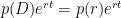
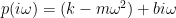
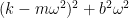
This solves (d), and with our values for $m$ , $b$ , and $k$ , it gives the answer to (b), $\omega_r=\sqrt{7}/3\simeq0.882$ .

(c) and (f) The complex gain is $1/p(i\omega)$ , so we are asked to find the angular frequency for which the real part of $p(i\omega)$ is zero and the imaginary part is positive. This occurs when $k=m\omega^2$ , or $\omega=\sqrt{k/m}$ (independent of $b$ !). With our values of $k$ and $m$ this gives $\omega=1$ .

(e) For $\omega_r$ to be real, the contents of the square root have to be non-negative. So $2mk\geq b^2$ .

This is a lot of computation and somewhat abstract. It is very reassuring to students to see the phenomena displayed on the Mathlet.

The complex gain is (in this problem) given by $1/p(i\omega)$ . The trajectory of this complex-valued function of $\omega$ is what is displayed in the [Nyquist plot]. It contains both the gain and the phase lag, and the Nyquist plot shows both and the relationship between them.

Technically, we have not drawn Bode plots: engineers would draw the log of the frequency horizontally, and the log of the gain vertically. My experience is that using log plots is a step too far for students at the stage at which I see them in my classes.

Also, a Nyquist plot, properly speaking, shows the trajectory of the complex gain for $\omega$ negative as well as positive.

For more Mathlets addressing these more advanced issues, see the Mathlets Bode and Nyquist Plots and Nyquist Plot.

Discussion Questions

Take a few moments to post a response in the following discussion forum. Once you have posted your responses, please read and respond to two of your classmates posts.

Module 3 Discussion Question 3: Secant Approximation Project Ideas
Module 3 Discussion Question 4: Frequency Response Project Ideas

Module 3 Resources

Mathlets-in-Homework-Slides.pdf

Module-3-Mathlets-in-Homework-Conclusion-Transcript.pdf

Module-3-Mathlets-in-Homework-Segment-1-Transcript.pdf